Walking Forward with Options

For a long time, I was intrigued by Darwinex’s YouTube video series on backtesting, overfitting, and methodologies for reducing overfitting risk. One of the approaches that stood out to me was walk-forward optimization.

If you are not familiar with the methodology, I recommend watching the video here (and the whole series here).

In short, walk-forward analysis (WFA) or walk-forward optimization (WFO) works by splitting historical data into a sequence of rolling windows, each consisting of an in-sample (IS) period followed by an out-of-sample (OOS) period.

For each window:

• You optimize your chosen parameters on the IS portion
• Then lock those parameters and test them on the immediately following OOS period

Once that’s done, the window rolls forward in time:

• A new IS window is formed (often overlapping with the previous one)
• Parameters are re-optimized
• And then validated again on the next OOS segment

This process repeats across the entire dataset, simulating how a strategy would be periodically re-optimized and deployed in real time, while continuously being tested on unseen data.

The goal is to ensure that the strategy adapts to changing market regimes without overfitting, by validating each set of parameters on data it hasn’t seen before.

The Setup

The challenge, of course, was that I could not realistically run such a rigorous test with the tools I had. Even a relatively simple WFO setup (33 = 9 combinations across 5 windows), like the one described in this post, requires about 50 backtests (45 in-sample tests, plus 5 additional out-of-sample tests). To run this without losing my mind to manual backtests, I built an automation platform that can set up and manage batch backtest tasks from template configurations (currently supporting WFO and parameter sweeps) based on a baseline portfolio. While it is still a work in progress, it already lets me produce results in minutes for a test I had virtually no way to run not too long ago.

There are many ways to configure this test, each with its own pros and cons, but here is how I chose to evaluate one of my strategies:

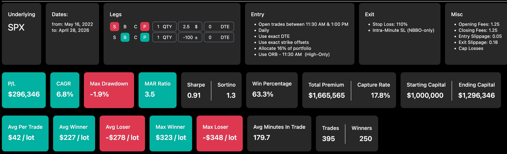
Selected my baseline backtest - I chose to run the test on my 0DTE 2H ORB PUT credit spread The strategy itself is quite simple - open a 100 wide put credit spread targeting 2.5$ premium whenever breaking the high of the 2 hours opening range and either take it to expiration (hopefully) or close at a loss of 110% of initial premium. Performance is very decent with a relatively high MAR, good PCR and a very manageable historical MDD in my taste.

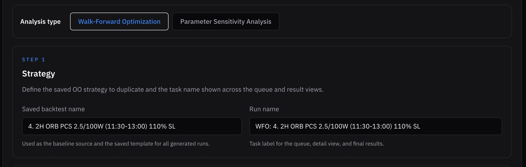
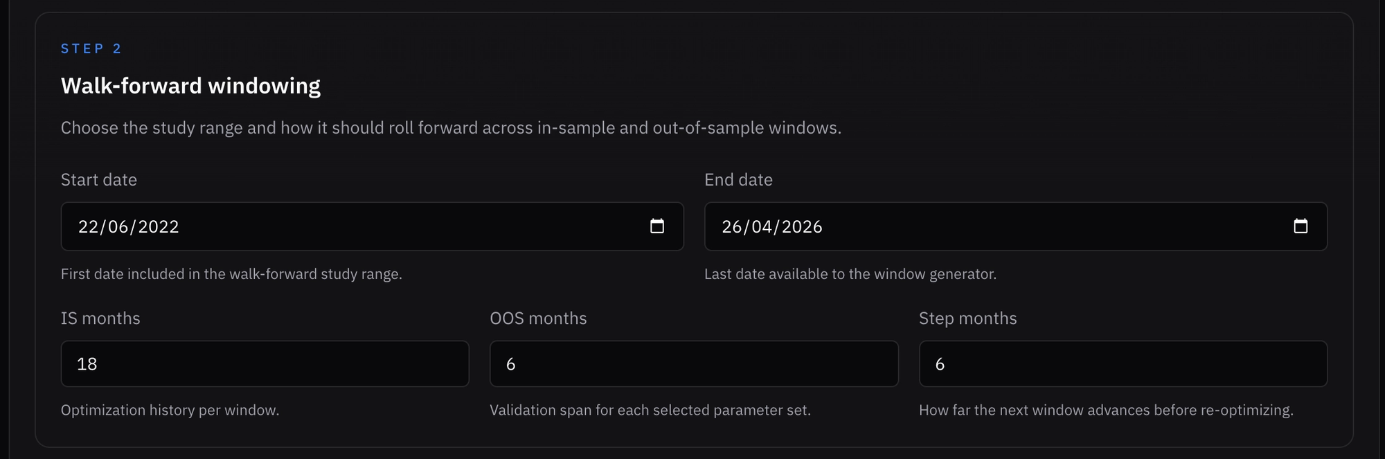
I decided to set window length to 18 months IS and 6 months OOS, with a step length of 6 months. This yields a 1:3 OOS to IS ratio and gives a good balance of statistical significance and enough difference between IS periods to better fit the changing regimes. Since this is a 0DTE trade, I set the period to start from SPX dailies.

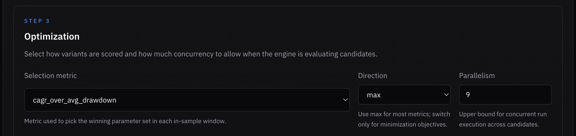
For IS optimization and the OOS validation metric, I chose CAGR over mean drawdown because it captures performance per unit of risk while also accounting for the severity of each drawdown (unlike MAR, which ignores drawdowns aside from the worst). This means “winning” in-sample parameters will be selected based on this metric, and walk-forward efficiency will be evaluated using the same metric.

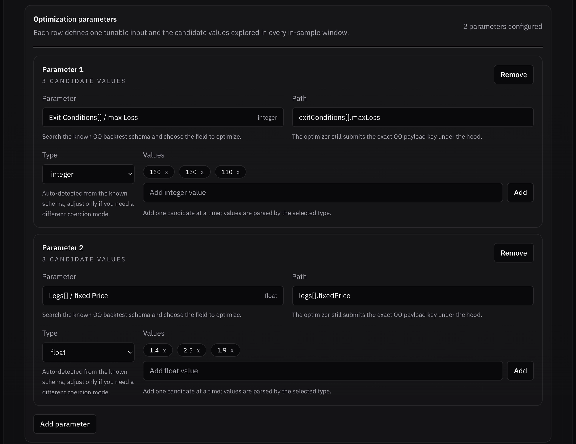
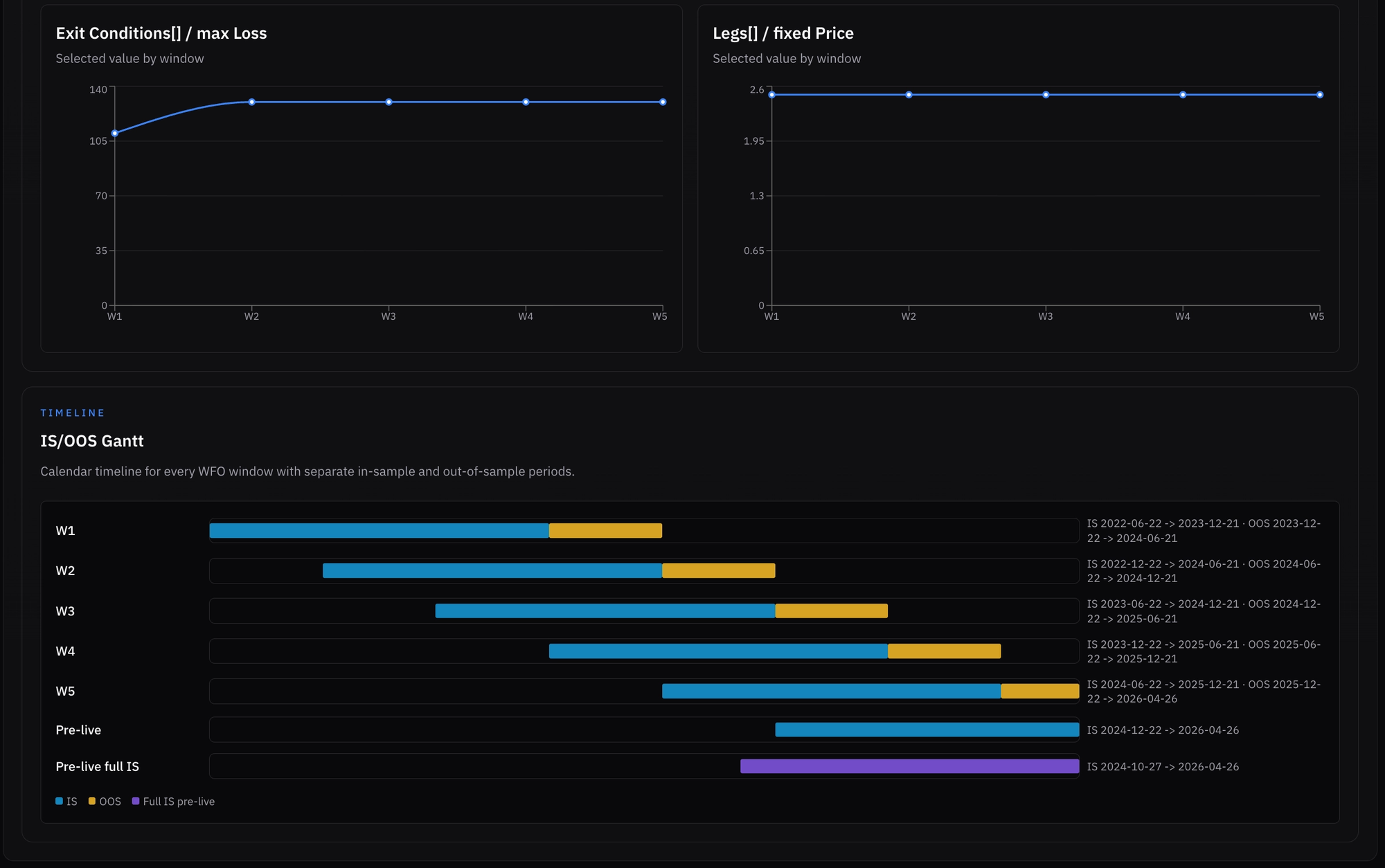
The chosen parameters and parameter values for the test were:

• Stop loss: 110%, 130%, 150%
• Credit target: 1.4, 1.9, 2.5
• Total combinations are therefore 3*3 = 9 for each in-sample period
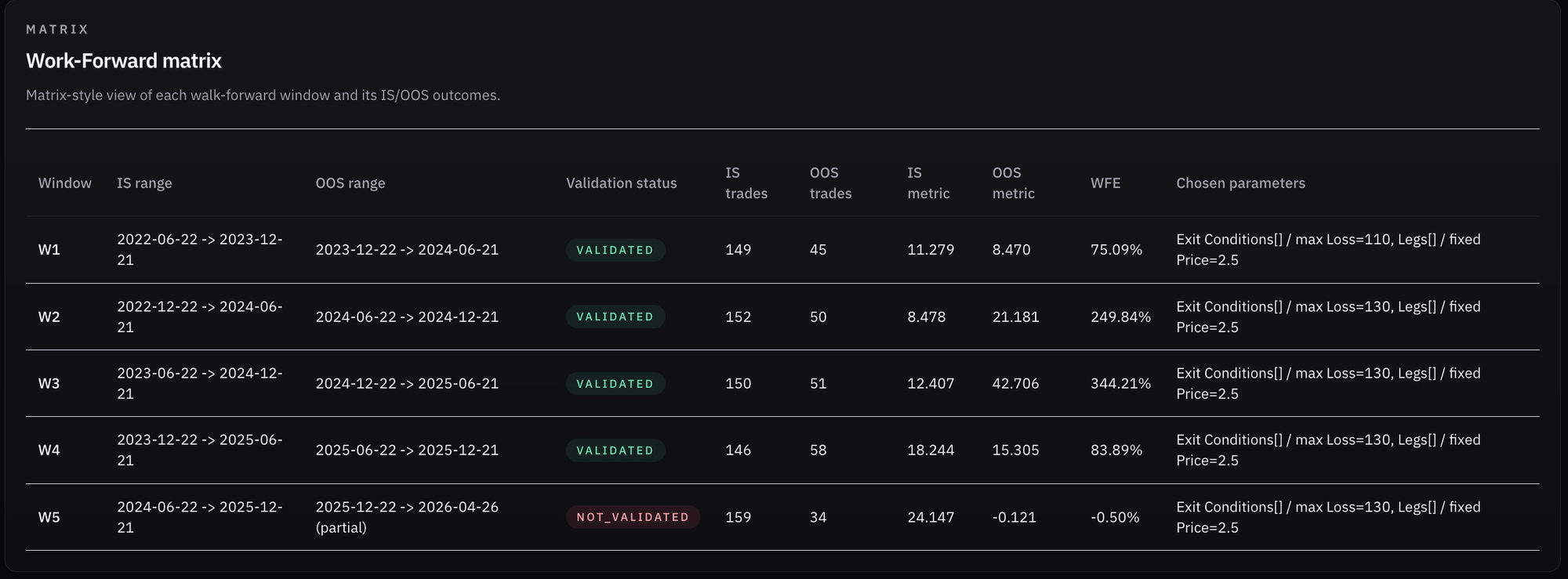
• Since the data was split into 5 windows, 9*5+5=50 total tests are run. All combinations are tested in each IS period, plus 5 additional OOS validation tests are run (one per window).

*I selected only 2 parameters and 3 values for each because you never want to over-optimize your strategies. Even with tools like WFO, you can still overfit to noise in each window, so reducing degrees of freedom helps generalization.

What this ultimately helps us assess:

• Does my strategy have valid predictive power? Do I see stability across OOS phases for all, or at least most, windows? (The selected comparison metric holds at least 50% of the metric value from the same window’s IS phase.) This is also called walk-forward efficiency.
• Is WFO helping improve performance and/or risk management? Does periodically re-optimizing the selected parameters improve long-term strategy performance when comparing the cumulative OOS results to the static backtest results?
• How many OOS periods were profitable out of the 100%?
• Is performance evenly distributed between windows, or do we have specific “lucky” windows? If so, how much do they contribute to overall performance?
• The end result is a “stitched” cumulative equity curve that combines all OOS periods from each window. This emulates “live” trading overall, since each OOS period is optimized based on its IS period and was never “contaminated” by overfitting. Therefore, the last IS window is effectively used as a “pre-live” optimization and dictates the parameter values to use for next live trading phase in the current market regime.

The Results!

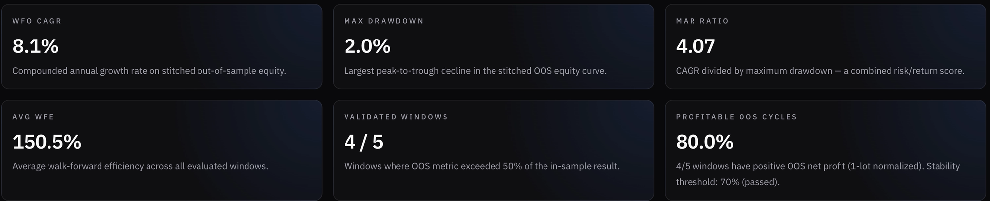
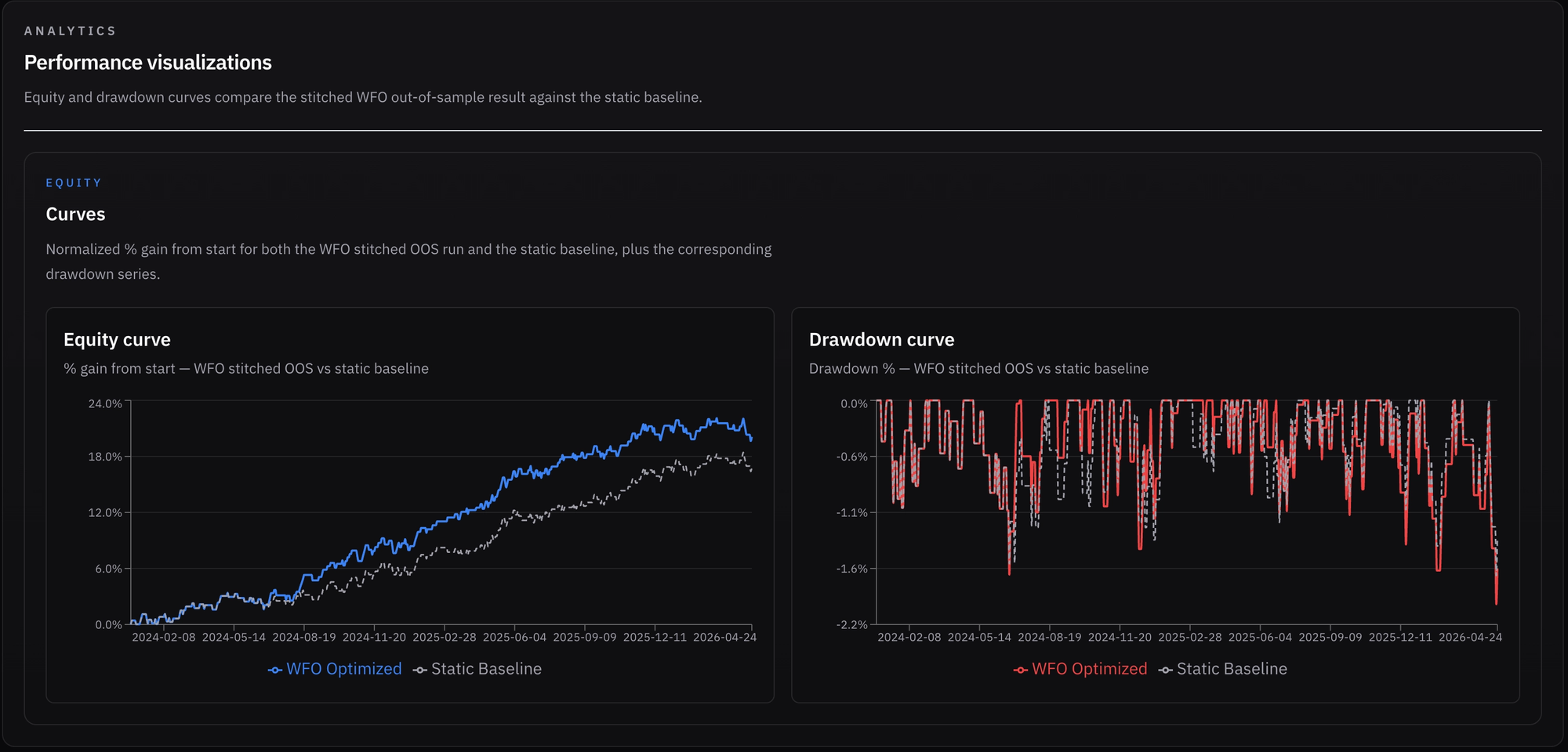
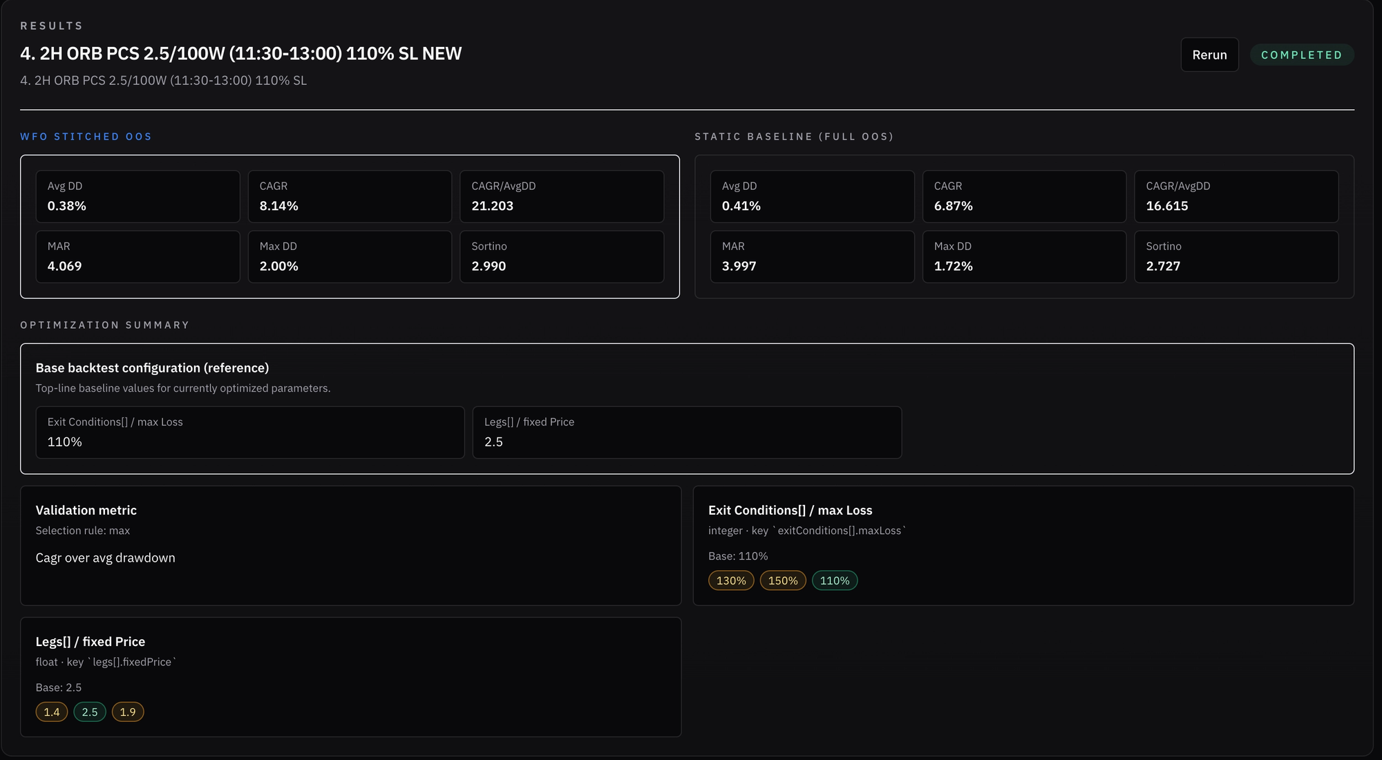
Right off the bat, I was excited to see that the test improved the results quite a bit. While MDD rose from 1.72% in the static backtest to 2%, average drawdown decreased slightly, and CAGR increased by 1.27%, from 6.87% to 8.14%!

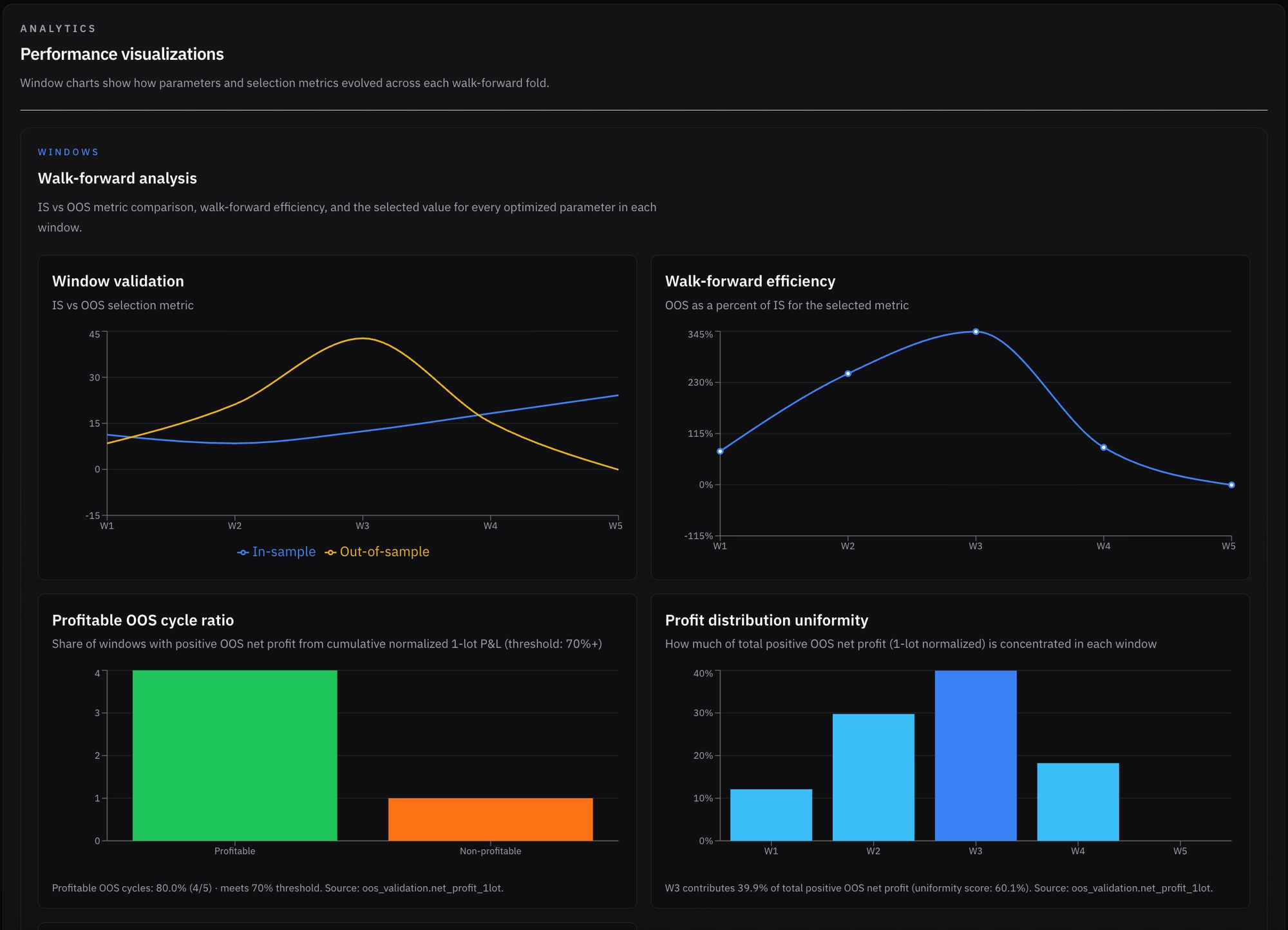
Looking at the results graphs, we can see what happened in each window and how stable the results were:

• We had ~150 IS trades per window and ~50 OOS trades (aside from the last window, which was truncated and had only 34 OOS trades).
• 2.5$ premium was selected for all windows, while the initial 110% stop loss was adjusted after the first window to 130%, and it kept winning and being selected for the rest of the tested windows.
• Aside from the most recent window, all windows were validated (the OOS period maintained at least 50% of the CAGR/mean DD from its IS period).
• Average walk-forward efficiency was 150%, which suggests strong predictive ability from IS to OOS. It is important to note that efficiency degrades in the last two windows, but the fourth window still has 83% efficiency, which is great. Some volatility is to be expected.
• Return distribution looked OK: the highest-return window contributed 40% of total normalized profits (data was normalized to avoid scaling skew), while the worst-performing window and the most recent, which was truncated, was relatively flat. The other three windows ranged from 12% to 30%. I suppose it is reasonable to expect any strategy’s performance to vary across different regimes. As long as risk is managed, I’m fine with it.
• MDD recently broke a record, but the same is true for the baseline backtest.

Pre-Live

Since I am still experimenting, I decided I want the platform to give me all recent winning parameters for different “versions” of the most recent in-sample (IS) run:

• The last window’s IS phase (5) - the one that produced the settings we are "currently" trading live during the truncated OOS period
• A pre-live IS using the set step after the last window (truncated in this case)
• A fresh full-length IS phase ending on the last day of the test, to capture the most recent regime fit

Here we could see all 3 variations' winners:

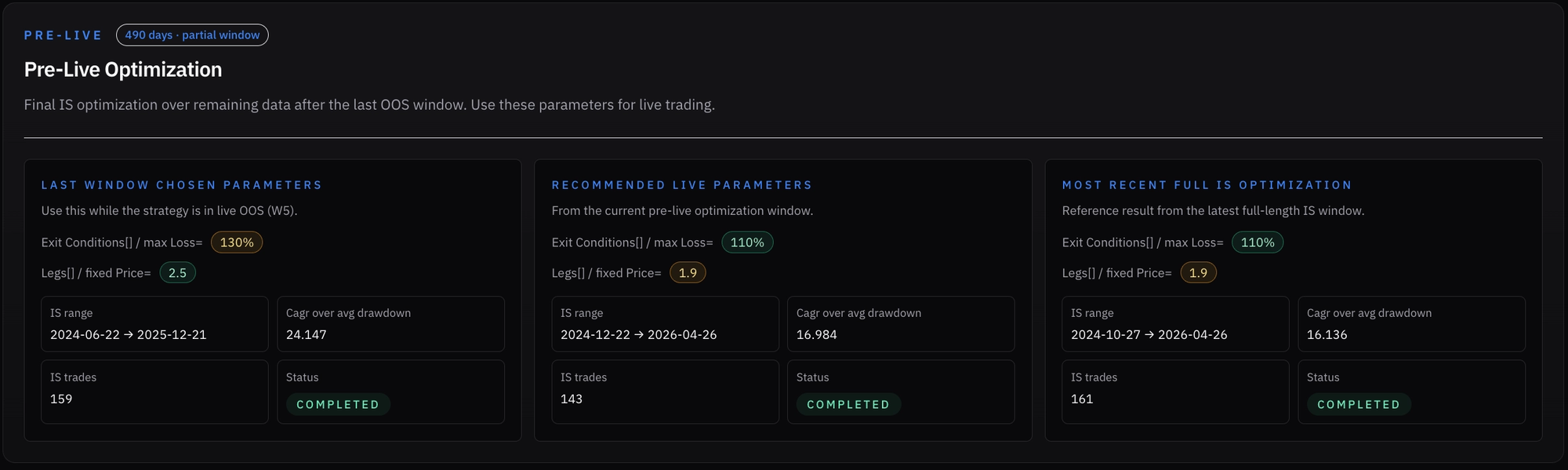
Interestingly, both the pre-live and full in-sample (IS) optimizations (which largely overlap) selected 1.9$ credit / 110% stop loss, while the most recent window we’re currently trading points to 2.5$ / 130% SL.

What makes this more interesting is that these parameters also differ from the broader historical behavior. The 2.5$ credit target has been the strongest performer overall across windows, while the 110% stop loss only appeared in the first window.

This leaves me with a decision to make:

• Continue trading using the current truncated OOS settings (2.5$/130%), finish the ongoing 6-month period, and only then re-optimize
• Treat this as a clean slate, and start the new live period with the 1.9$/110% configuration
• Run a fresh WFO with adjusted windowing so the historical data is split more cleanly - avoiding OOS truncation and ensuring the final IS phase aligns exactly with the pre-live period

Some important caveats and notes:

• Statistical significance is always something to consider. With a limited trade count since dailies, you want each in-sample window to have more trades (higher degrees of freedom). I felt more comfortable with ~150 trades per in-sample window. Generally speaking, the OOS period requires fewer trades because it uses no degrees of freedom and is used for validation.
• Window size, and especially step size, matters because it determines how different the market regimes are between optimization periods. If these are too small, the process may not capture meaningful regime changes to optimize for.
• The choice of parameters to optimize, the values tested, and the validation metric are all crucial and can dramatically impact the results. It’s therefore important to do proper due diligence and select options that genuinely make sense. Understanding the trade’s profit mechanisms, the market environment, and the expected behavior of the Greeks is always important and can help guide these decisions. Here, I chose to optimize the credit target and the stop-loss size since the only other potential candidates to optimize are spread size and opening range time which I decided to keep constant. For the credit target, the idea was that different market regimes may favor higher or lower premium collection, effectively shifting the spread further OTM or ITM depending on conditions. As for the stop loss, I assumed the strategy could benefit from being more adaptive, tightening or loosening risk management based on what the market environment rewards at the time.
• Some strategies may show degradation in long-term results. Not all strategies benefit from this method.
• This method requires periodic re-optimization for live trading based on the set step size - the end result is a series of actual live “OOS” windows which together comprises your live trading.

Final Thoughts

Walk-forward analysis is a powerful tool because it allows you to use historical data more efficiently. In a standard IS/OOS split, you typically allocate only 25%–33% of the data to out-of-sample in order to preserve a sufficiently large in-sample dataset for optimization.

With WFO, you effectively get the best of both worlds. You maintain a similar IS-to-OOS ratio per window, while rolling that process forward through time. This results in more than 50% non-overlapping out-of-sample data, while still benefiting from a sufficiently large in-sample dataset for each optimization phase.

Another thing I really like about this method is that it better reflects real trading conditions. Strategies that fail to remain consistent across multiple out-of-sample phases often point to a weak edge or signs of overfitting.

For certain strategies, as we saw here, this approach can meaningfully improve long-term results.

Even if it doesn’t improve raw performance, it helps you estimate the true robustness of a strategy before risking real capital - and gives you a more realistic sense of whether future results are likely to follow a similar statistical pattern.

I am definitely going to run this test on more strategies and keep you all updated.